Last-Minute Study Guide

Tresca (maximum shear stress) — yielding starts when the largest shear stress equals the tension-test shear value \(\sigma_y/2\):

\[ \tau_{\max}=\frac{\sigma_1-\sigma_3}{2}=\frac{\sigma_y}{2}\;\Longrightarrow\; \sigma_1-\sigma_3=\sigma_y \]

von Mises (distortion energy) — general 3-D and the biaxial case \(\sigma_3=0\):

\[ \sigma'=\sqrt{\tfrac12\big[(\sigma_1-\sigma_2)^2+(\sigma_2-\sigma_3)^2+(\sigma_3-\sigma_1)^2\big]}\ge\sigma_y,\qquad \sigma'_{\text{biaxial}}=\sqrt{\sigma_1^2-\sigma_1\sigma_2+\sigma_2^2} \]

• \(\sigma_1\ge\sigma_2\ge\sigma_3\) = the three principal stresses (largest → smallest), MPa
• \(\sigma_y\) = uniaxial tensile yield strength of the material, MPa
• \(\sigma'\) = von Mises "equivalent" stress — one number that stands in for the whole stress state
• \(\tau_{\max}\) = maximum shear stress in the element, MPa

How to use: find the principal stresses, plug into a criterion, and yielding is predicted the moment the left side reaches \(\sigma_y\). Factor of safety \(n=\sigma_y/\sigma'\) (von Mises) or \(n=\sigma_y/(\sigma_1-\sigma_3)\) (Tresca).

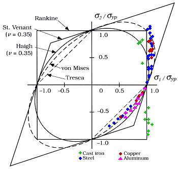
The five yield surfaces individually (course slides): a point inside is safe, on the boundary it yields.

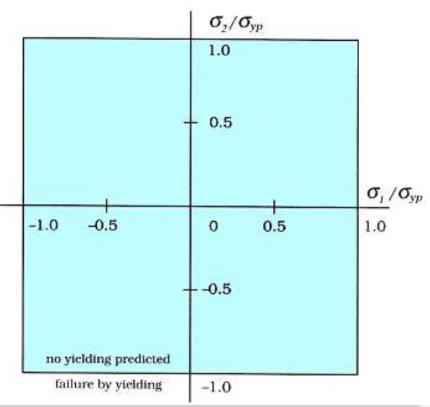
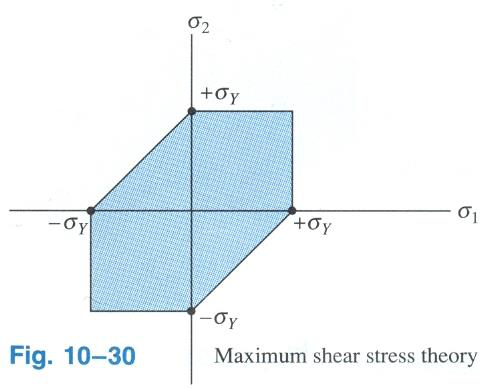
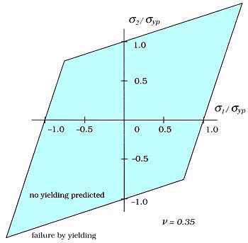
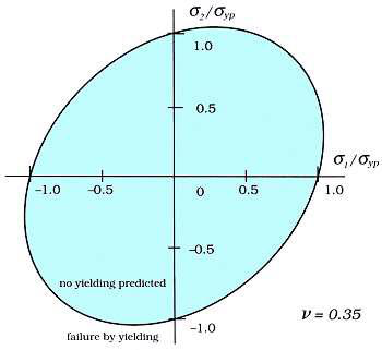
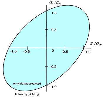
Any stress point inside a surface is safe; on the surface it yields. Because the Tresca hexagon lies inside the von Mises ellipse, Tresca reaches its boundary sooner → it predicts yielding at a lower load → it is the safer / more conservative theory. Von Mises is less conservative but matches experiment better.

Total strain energy splits into a volumetric part (change of size, driven by hydrostatic stress) and a distortional part (change of shape). Experiments show hydrostatic pressure alone does not yield metals, so only the distortion energy should count toward yield — which is exactly what von Mises measures. That physical reasoning is why it beats both Tresca and the total-strain-energy (Haigh) theory.

The stress at a point has 9 components; symmetry \(\tau_{ij}=\tau_{ji}\) leaves 6 independent (3 normal + 3 shear):

\[ \sigma_{ij}=\begin{bmatrix}\sigma_{xx}&\tau_{xy}&\tau_{xz}\\ \tau_{yx}&\sigma_{yy}&\tau_{yz}\\ \tau_{zx}&\tau_{zy}&\sigma_{zz}\end{bmatrix} \]

Generalized Hooke's law (isotropic, linear-elastic), plus the shear modulus link:

\[ \varepsilon_x=\frac1E\big[\sigma_x-\nu(\sigma_y+\sigma_z)\big]\ (\text{+ cyclic}),\qquad \gamma_{xy}=\frac{\tau_{xy}}{G},\qquad G=\frac{E}{2(1+\nu)} \]

• \(\sigma,\tau\) = normal and shear stresses (MPa); \(\varepsilon,\gamma\) = normal and shear strains
• \(E\) = Young's modulus, \(\nu\) = Poisson's ratio, \(G\) = shear modulus

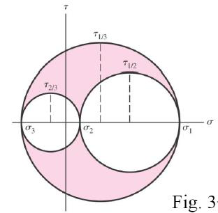
Principal planes carry no shear; their normal stresses are the principal stresses.

\[ \sigma_{1,2}=\frac{\sigma_x+\sigma_y}{2}\pm\sqrt{\left(\frac{\sigma_x-\sigma_y}{2}\right)^2+\tau_{xy}^2},\qquad \tau_{\max}=\sqrt{\left(\frac{\sigma_x-\sigma_y}{2}\right)^2+\tau_{xy}^2} \] \[ \tan 2\theta_p=\frac{2\tau_{xy}}{\sigma_x-\sigma_y} \]

• \(\sigma_x,\sigma_y\) = normal stresses on the x- and y-faces; \(\tau_{xy}\) = shear on those faces
• \(\theta_p\) = angle from the x-axis to a principal plane; on Mohr's circle a physical rotation \(\theta\) appears as \(2\theta\)
• centre = \((\sigma_x+\sigma_y)/2=\sigma_{avg}\); radius = \(\tau_{\max}\)

How to use: the first term is the circle's centre, the square-root is its radius; \(\sigma_{1,2}=\)centre \(\pm\) radius.

\[ \text{Flexure: }\frac{M}{I}=\frac{\sigma_b}{y}=\frac{E}{\rho}\qquad \text{Torsion: }\frac{T}{J}=\frac{\tau}{\rho}=\frac{G\phi}{L},\quad J=\frac{\pi}{32}(D^4-d^4) \]

• \(M\) = bending moment, \(I\) = second moment of area, \(y\) = distance from neutral axis, \(\rho\) = radius of curvature
• \(T\) = torque, \(J\) = polar second moment, \(\phi\) = angle of twist, \(L\) = length, \(D,d\) = outer/inner diameter

Traditional design compares stress to strength (2 parameters). A crack doesn't create stress — it intensifies the far-field stress at its tip; the sharper the tip, the higher the local stress. Fracture mechanics adds flaw size as a third parameter and asks: what is the strength as a function of crack size, and what is the largest tolerable crack?

Near the tip the stress field scales as \(K/\sqrt{2\pi r}\). The design number is the stress-intensity factor \(K_I\); fracture occurs when it reaches the fracture toughness \(K_{IC}\):

\[ K_I=Y\,\sigma\sqrt{\pi a}\quad(\text{fracture when }K_I\ge K_{IC})\qquad\Longrightarrow\qquad a_c=\frac{1}{\pi}\left(\frac{K_{IC}}{Y\sigma}\right)^2 \]

• \(K_I\) = Mode-I stress-intensity factor (MPa·√m) — the crack "driving" quantity
• \(Y\) = geometry factor (1.0 central crack, 1.12 edge, 0.64 penny)
• \(\sigma\) = remote applied stress (MPa); \(a\) = crack length in metres (half-length for a central crack, full for an edge crack)
• \(K_{IC}\) = plane-strain fracture toughness (material property); \(a_c\) = critical crack length at which fracture begins

How to use: compute \(K_I\) for the actual crack; safe while \(K_I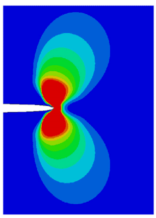

Griffith (ideally brittle): a crack grows when the strain energy released \(\ge\) the energy to create new crack surface. Irwin–Orowan adds plastic work \(\gamma_p\) for metals \((\gamma_s\to\gamma_s+\gamma_p,\ \gamma_p\gg\gamma_s)\) — why tough steel absorbs far more than its bond energy.

\[ \frac{dU_s}{da}\ge\frac{dU_\gamma}{da},\quad U_s=\frac{\pi a^2\sigma^2}{E},\ U_\gamma=4\gamma_s a\ \Longrightarrow\ \sigma_f=\sqrt{\frac{2E\gamma_s}{\pi a}} \]

The energy release rate \(G\) links energy and \(K\):

\[ G=\frac{K_I^2}{E'}\qquad(E'=E\text{ plane stress};\ E'=E/(1-\nu^2)\text{ plane strain}) \]

• \(U_s\) = elastic strain energy released; \(U_\gamma\) = surface energy consumed
• \(\gamma_s\) = surface energy per unit area; \(\sigma_f\) = fracture stress; \(G\) = energy released per unit crack extension (crack "driving force")

\[ \sigma_a=\frac{\sigma_{max}-\sigma_{min}}{2},\quad \sigma_m=\frac{\sigma_{max}+\sigma_{min}}{2},\quad \Delta\sigma=\sigma_{max}-\sigma_{min},\quad R=\frac{\sigma_{min}}{\sigma_{max}} \]

• \(\sigma_a\) = amplitude (drives fatigue); \(\sigma_m\) = mean stress; \(\Delta\sigma\) = stress range; \(R\) = stress ratio
• Fully reversed \(R=-1\ (\sigma_m=0)\); repeated \(R=0\ (\sigma_{min}=0)\); fluctuating \(0

\[ S_a=a\,N^{\,b}\ (b<0)\quad\Rightarrow\quad \frac{S_1}{S_2}=\left(\frac{N_1}{N_2}\right)^{b} \]

• \(S_a\) = stress amplitude for life \(N\); \(N\) = cycles to failure
• \(a\) = fatigue-strength coefficient (intercept); \(b\) = fatigue-strength exponent (slope, negative)

How to use: if you know one point \((S_1,N_1)\) and \(b\), the ratio form gives the strength at any other life \(N_2\) without finding \(a\).

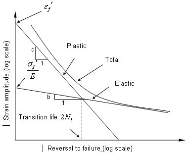
Region II of the \(da/dN\)–\(\Delta K\) curve is linear on log–log axes. Use the stress range \(\Delta\sigma\):

\[ \Delta K=Y\,\Delta\sigma\sqrt{\pi a},\qquad \frac{da}{dN}=C(\Delta K)^m \] \[ N=\int_{a_i}^{a_f}\frac{da}{C\,(Y\Delta\sigma\sqrt{\pi a})^m}\ \xrightarrow{\,m=3\,}\ N=\frac{2\big[a_i^{-1/2}-a_f^{-1/2}\big]}{C\,(Y\Delta\sigma\sqrt{\pi})^{3}} \]

• \(da/dN\) = crack growth per cycle (m/cycle); \(\Delta K\) = stress-intensity range
• \(C,m\) = Paris material constants (\(m\approx3\) for steels); \(a_i,a_f\) = initial & final (critical) crack lengths

How to use: get \(a_f=a_c\) from \(K_{IC}\), then plug into the \(m=3\) result. Keep \(a\) in metres and use \(\Delta\sigma\), never \(\sigma_{max}\).

\[ D=\sum_i\frac{n_i}{N_i};\qquad\text{failure when }D\ge1\quad(\text{blocks to failure}=1/D) \]

• \(n_i\) = cycles applied at stress level \(i\); \(N_i\) = cycles to failure at that level; \(D\) = accumulated damage

\[ R(t)=1-F(t),\qquad \lambda(t)=\frac{f(t)}{R(t)},\qquad \lambda=\frac{\text{failures}}{\text{operating time}} \] \[ \text{MTTF}=\int_0^\infty R(t)\,dt=\frac1\lambda\ (\text{non-repairable}),\qquad \text{MTBF}=\frac1\lambda\ (\text{repairable}) \]

• \(R(t)\) = reliability (probability of surviving to \(t\)); \(F(t)\) = unreliability (CDF); \(f(t)\) = failure PDF
• \(\lambda\) = hazard / failure rate; MTTF = mean time to failure; MTBF = mean time between failures

\[ \text{Exponential: }R=e^{-\lambda t}\qquad \text{Normal: }R=1-\Phi\!\left(\tfrac{t-\mu}{\sigma}\right)\qquad \text{Weibull: }R=e^{-(t/\theta)^m} \] \[ \text{Series (all needed): }R_s=\prod R_i\qquad \text{Parallel (any one): }R_s=1-\prod(1-R_i) \]

• \(\mu,\sigma\) = mean & std-dev (Normal); \(\theta\) = characteristic life, \(m\ (\equiv\beta)\) = Weibull shape

Both stress and strength are distributions, not single values. Where the tails overlap, an item sees a stress above its strength → failure. The overlap area is the probability of failure; the gap between the means is the safety margin.

DFR levers: increase the margin, derate, add redundancy, reduce scatter (better QC) — all shrink the overlap.

\[ n=\frac{S}{\sigma}=\frac{\text{Strength}}{\text{Stress}} \]

The design factor \(n_d\) is the target chosen before sizing, to cover uncertainty in material, load and analysis. The factor of safety is the margin you actually end up with after rounding dimensions up to standard sizes. Stress and strength must be the same type, units and location.